BAITS.IR module

Import packages

import os
import numpy as np
import pandas as pd
import seaborn as sns
import matplotlib.pyplot as plt
from scipy.stats import pearsonr

import BAITS

Import files

Users could read the example data from the github, also could access the data through the link

bcr_loc_df = pd.read_csv('../data/bcr_sampled.tsv', sep='\t', index_col=0)
bcr_loc_df.head(n=2) 

	sample	bcUmi	clone	aaClone	Vgene	Jgene	Cgene	cdr3nt
0	P0516-LM	E14D5FEFEBE3D5C47	TGTCAACAGAGTCACAGTATACCTACTTTT_CQQSHSIPTF_IGKV...	CQQSHSIPTF_IGKV1-39_IGKJ2_IGK	IGKV1-39	IGKJ2	IGK	TGTCAACAGAGTCACAGTATACCTACTTTT
1	P0516-LM	8E153B79054792CA2	TGTCAACAATATAGCACTGTCCCCCTCACTTTC_CQQYSTVPLTF_...	CQQYSTVPLTF_IGKV1-27_IGKJ4_IGK	IGKV1-27	IGKJ4	IGK	TGTCAACAATATAGCACTGTCCCCCTCACTTTC

Define parameters

sample_col = 'sample'
Umi_col = 'bcUmi'
clone_col = 'clone'
cdr3nt_col = 'cdr3nt'
Vgene_col = 'Vgene'
Jgene_col = 'Jgene'
Cgene_col = 'Cgene'

Quality Control

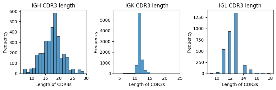
Calculate clonal CDR3 length

Here, BAITS provides functions to calculate and visualize the length distribution of CDR3 region. The cauculated results will be returned.

bcr_loc_df = BAITS.VDJ.tl.calculate_cdr3_length(bcr_loc_df, sample_col, Cgene_col, cdr3nt_col, cdr3_type='nt', plot=True)

bcr_loc_df.head(n=2) 

	sample	bcUmi	clone	aaClone	Vgene	Jgene	Cgene	cdr3nt	cdr3_length
0	P0516-LM	E14D5FEFEBE3D5C47	TGTCAACAGAGTCACAGTATACCTACTTTT_CQQSHSIPTF_IGKV...	CQQSHSIPTF_IGKV1-39_IGKJ2_IGK	IGKV1-39	IGKJ2	IGK	TGTCAACAGAGTCACAGTATACCTACTTTT	10
1	P0516-LM	8E153B79054792CA2	TGTCAACAATATAGCACTGTCCCCCTCACTTTC_CQQYSTVPLTF_...	CQQYSTVPLTF_IGKV1-27_IGKJ4_IGK	IGKV1-27	IGKJ4	IGK	TGTCAACAATATAGCACTGTCCCCCTCACTTTC	11

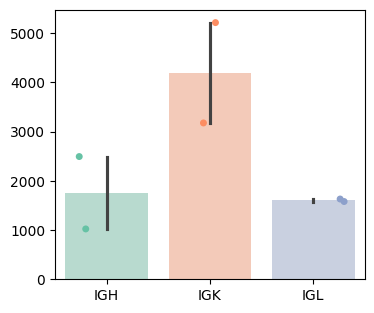
Calculate clonal richness

BAITS provides function to calculate and visualize the clonal number per sample

bcr_loc_df = BAITS.VDJ.tl.stat_clone(bcr_loc_df, 'sample', Cgene_col, clone_col) 

bcr_loc_df.head(n=2) 

	sample	bcUmi	clone	aaClone	Vgene	Jgene	Cgene	cdr3nt	cdr3_length	clone_by_sample
0	P0516-LM	E14D5FEFEBE3D5C47	TGTCAACAGAGTCACAGTATACCTACTTTT_CQQSHSIPTF_IGKV...	CQQSHSIPTF_IGKV1-39_IGKJ2_IGK	IGKV1-39	IGKJ2	IGK	TGTCAACAGAGTCACAGTATACCTACTTTT	10	5216
1	P0516-LM	8E153B79054792CA2	TGTCAACAATATAGCACTGTCCCCCTCACTTTC_CQQYSTVPLTF_...	CQQYSTVPLTF_IGKV1-27_IGKJ4_IGK	IGKV1-27	IGKJ4	IGK	TGTCAACAATATAGCACTGTCCCCCTCACTTTC	11	5216

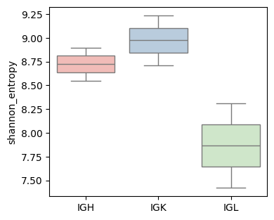
Calculate immune repertoire features

Calculates the Shannon entropy of the CDR3 repertoire, leveraging UMI information to correct for sequencing errors and amplification bias.

groups = [sample_col, Cgene_col] # user-customizable based on experimental design

shannon_entropy_df = BAITS.VDJ.tl.compute_grouped_index(bcr_loc_df, sample_col, Cgene_col, clone_col, groups, count_basis = 'UMI', Umi_col='bcUmi', index='shannon_entropy')

Here, the Shannon entropy of the CDR3 repertoire is computed, stratified by both sample and C gene (chain type) groups.

shannon_entropy_df.head()

	sample	Cgene	shannon_entropy
0	P0516-LM	IGH	8.898825
1	P0516-LM	IGK	9.235398
2	P0516-LM	IGL	8.314985
3	P1128-LM	IGH	8.548061
4	P1128-LM	IGK	8.711763

fig, ax = plt.subplots(1,1,figsize=(4, 3.5))
BAITS.VDJ.pl._boxplot(shannon_entropy_df, 'Cgene', 'shannon_entropy', groupby='Cgene', palette='Pastel1', xlabel=None, ylabel='shannon_entropy', log=False, ax=ax )
plt.show()

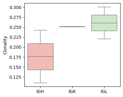
Calculates the Clonality of the CDR3 repertoire, leveraging UMI information to correct for sequencing errors and amplification bias.

Clonality quantifies the unevenness of clonal frequencies in the immune repertoire. Higher clonality suggests antigen-driven expansion and potential immune dominance

groups = [sample_col, Cgene_col]
shannon_entropy_df = BAITS.VDJ.tl.compute_grouped_index(bcr_loc_df, sample_col, Cgene_col, clone_col, groups, count_basis = 'UMI', Umi_col='bcUmi', index='Clonality')

fig, ax = plt.subplots(1,1,figsize=(4, 3.5))
BAITS.VDJ.pl._boxplot(shannon_entropy_df, 'Cgene', 'Clonality', groupby='Cgene', palette='Pastel1', xlabel=None, ylabel='Clonality', log=False, ax=ax )
plt.show()

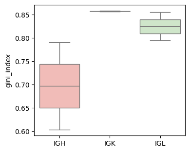
Gini_index (based on UMIs)

groups = [sample_col, Cgene_col]
gini_index_df = BAITS.VDJ.tl.compute_grouped_index(bcr_loc_df, sample_col, Cgene_col, clone_col, groups, count_basis = 'UMI', Umi_col='bcUmi', index='gini_index')
gini_index_df['tissue'] = gini_index_df['sample'].str.split('-').str[1]

fig, ax = plt.subplots(1,1,figsize=(4, 3.5))
BAITS.VDJ.pl._boxplot(gini_index_df, 'Cgene', 'gini_index', groupby='Cgene', palette='Pastel1', xlabel=None, ylabel='gini_index', log=False, ax=ax )
plt.show()

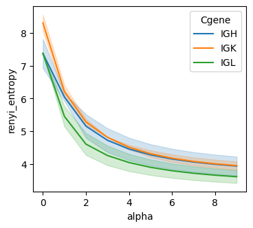
Renyi_entropy (based on UMIs)

Renyi entropy is a generalized diversity measure that captures different aspects of repertoire structure through an adjustable parameter alpha.

groups = [sample_col, Cgene_col]
renyi_entropy_df = BAITS.VDJ.tl.compute_grouped_index(bcr_loc_df, sample_col, Cgene_col, clone_col, groups, count_basis = 'UMI', Umi_col='bcUmi', index='renyi_entropy')

fig, ax = plt.subplots(1,1,figsize=(4, 3.5))
sns.lineplot(data=renyi_entropy_df, x="alpha", y="renyi_entropy", hue='Cgene', ax=ax )
plt.show()

Cluster BCR sequences to get BCR family

We first focus on IGH BCRs (Immunoglobulin Heavy Chains) because they are the most important for analyzing BCR clusters and clonal families. By selecting only rows where the Cgene column equals ‘IGH’, we create a subset of the data that contains only IGH sequences, which will be used for downstream clustering and diversity analysis.

igh_bcr_loc_df = bcr_loc_df[bcr_loc_df['Cgene']=='IGH'].copy()

BCR sequences are first grouped by V gene, J gene, and CDR3 length. Within each group, sequences sharing ≥85% nucleotide identity (user-defined) are seen from the same BCR family.

igh_bcr_loc_df = BAITS.VDJ.tl.cluster_bcrs(igh_bcr_loc_df, threshold=0.85, sample_col='sample',  Vgene_col='Vgene', Jgene_col='Jgene', cdr3nt_col='cdr3nt')

igh_bcr_loc_df.iloc[:,-5:].head() 

	cdr3_length	clone_by_sample	CDR3_nt_length	BCR_familyID	Degree
0	13	1023	39	IGHV1-45_IGHJ4_39_0	0
1	20	1023	60	IGHV4-4_IGHJ5_60_0	0
2	14	1023	42	IGHV4-39_IGHJ4_42_2	0
3	21	1023	63	IGHV3-72_IGHJ4_63_0	1
4	18	1023	54	IGHV1-69_IGHJ6_54_1	0

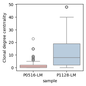
Degree centrality

Clonal degree centrality: Measure of the number of similar clones (with a hamming distance ≤ 1) connected to each unique V(D)J sequence within a clonal family. A high degree centrality value suggests that a particular V(D)J sequence serves as a progenitor clone, from which multiple related sequences have diverged via somatic hypermutation. This pattern is indicative of active antigen-driven diversification and affinity maturation. Conversely, a low degree centrality value indicates that the sequence is peripheral or isolated within the clonal network, with few connected variants. This may suggest limited subsequent diversification, potentially representing either a recently emerged clone or one that has not undergone significant antigen-driven expansion.

plt.subplots(1,1,figsize=(3, 3))
sns.boxplot(igh_bcr_loc_df, x='sample', y='Degree', palette='Pastel1')
plt.ylabel('Clonal degree centrrality')
plt.show()

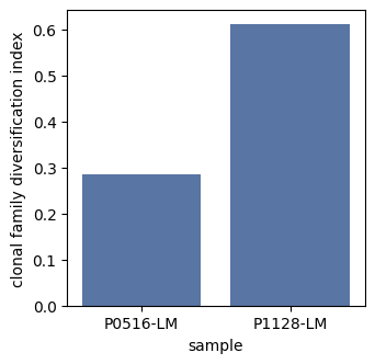
Calculate clonal family diversification index

Clonal family diversification: Measures the unevenness in the distribution of unique V(D)J sequences across clonal families using the Gini index. A high value indicates that certain clonal families contain numerous distinct V(D)J sequences – a pattern often associated with antigen-driven expansion and diversification.

Clonal_family_diver_idx = BAITS.VDJ.tl.Clonal_family_diversification(igh_bcr_loc_df, sample_col='sample', cluster_col='BCR_familyID', cdr3_col='cdr3nt') 
    
Clonal_family_diver_idx.head()

	sample	Clonal_family_diver_index
0	P0516-LM	0.285553
1	P1128-LM	0.611375

plt.subplots(1,1,figsize=(3.5, 3.5))
sns.barplot(Clonal_family_diver_idx,x='sample', y='Clonal_family_diver_index', color='#4C72B0')
plt.ylabel('clonal family diversification index')
plt.show()