BAITS.st.module - Spatial clustering#
Except for clustering the spatially close cells, we can also cluster the gene-expression similar domains. In this part, we will spatial cluster the domains based on CellCharter.
Import packages and data#
import os
import anndata as ad
import numpy as np
import scanpy as sc
import matplotlib.pyplot as plt
import matplotlib.image as mpimg

import BAITS
Users could access the data through the following link
adata = sc.read("./data/twosamples.h5ad")
adata
AnnData object with n_obs × n_vars = 968003 × 25091
    obs: 'n_genes_by_counts', 'total_counts', 'pct_counts_mt', 'celltype', 'sample', 'Bcell_enrichment'
    var: 'mt'
    obsm: 'spatial'
# Normalizing to median total counts
sc.pp.normalize_total(adata)

# Logarithmize the data
sc.pp.log1p(adata)
Gene expression matrix process#
Dimensionality reduction - Reduce the dimensionality of the data by running principal component analysis (PCA), which reveals the main axes of variation and denoises the data.
sc.tl.pca(adata)
Integrating gene expression matrices across multiple samples and removing batch effects
sc.external.pp.harmony_integrate(adata, key='sample', basis='X_pca' )
adata
AnnData object with n_obs × n_vars = 968003 × 25091
    obs: 'n_genes_by_counts', 'total_counts', 'pct_counts_mt', 'celltype', 'sample', 'Bcell_enrichment'
    var: 'mt'
    uns: 'log1p', 'pca'
    obsm: 'spatial', 'X_pca', 'X_pca_harmony'
    varm: 'PCs'
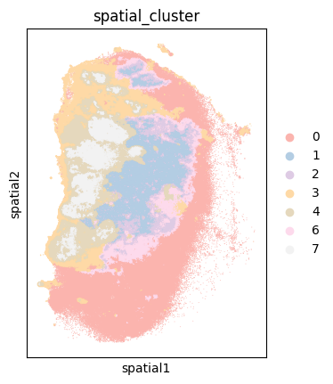
Spatial clustering#
We next computed spatial clusters by constructing networks for the cells in each sample. In these networks, each cell is encoded as a node, and an edge connects two cells if they are in close physical proximity within the tissue.
BAITS.st.gr.spatial_neighbors(adata, sample_key='sample', coord_type='generic', delaunay=True, spatial_key='spatial')
The next step is the neighborhood aggregation. It consists of concatenating the features of every cell with the features aggregated from neighbors ad increasing layers from the considered cell, up to a certain layer n_layers. Aggregation functions are used to obtain a single feature vector from the vectors of multiple neighbors, with the default being the mean function.
In this case we use 3 layers of neighbors. That is the cell’s reduced vector size from PCA plus the aggregated vectors from the 3 layers of neighbors.
BAITS.st.gr.aggregate_neighbors(adata, n_layers=3, use_rep='X_pca')
We create the Gaussian Mixture model, specifying 10 as desired number of clusters.
gmm = BAITS.st.tl.Cluster(
    n_clusters=10, random_state=12345,
    # If running on GPU
    # trainer_params=dict(accelerator='gpu', devices=1)
)
gmm.fit(adata, use_rep='X_cellcharter')
adata.obs['spatial_cluster'] = gmm.predict(adata, use_rep='X_cellcharter')
sc.pl.spatial(adata[adata.obs['sample']=='P0516_LM'], color=['spatial_cluster'], spot_size=50, palette='Pastel1')
Additionally, an H&E-stained image from the same sample is available for visualization.
img = mpimg.imread('./data/P0516_LM_HE.tif')
plt.imshow(img)
plt.axis('off')
plt.show()
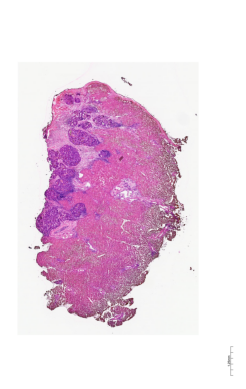
A comparison of the spatial clustering result with the corresponding H&E image reveals a high degree of confidence in the clustering outcome.