BAITS.st.module - Identify BLAs

This tutorial shows an example of B lymphocyte aggregates (BLAs) identification. The dataset is composed of 2 human liver metastatic colorectal tumor samples profiled by Stereo-seq from originial paper.

Import packages and data

import os
import BAITS
import anndata as ad
import numpy as np
import scanpy as sc

Users could access the data through the following link

adata = sc.read("./twosamples.h5ad") 

adata

AnnData object with n_obs × n_vars = 968003 × 25091
    obs: 'n_genes_by_counts', 'total_counts', 'pct_counts_mt', 'celltype', 'sample'
    var: 'mt'
    obsm: 'spatial'

# Normalizing to median total counts
sc.pp.normalize_total(adata)

# Logarithmize the data
sc.pp.log1p(adata)

Identify B lymphocytes enriched regions

To identify B cell-enriched regions in spatial transcriptomics data, we defined a custom gene signature. This signature was used to calculate an enrichment score for each spot, allowing for the spatial mapping of B cell locales.

signature = ["CD79A", "CD79B", "MS4A1", "CD79A", 'CD79B', "MZB1", "JCHAIN", "IGHA1", 'IGHG1', 'IGHG3']

Custom score name

score_name = 'Bcell_enrichment'

The user must provide the name of the column in adata.obs that identifies samples. Based on this parameter, BAITS performs integration by processing each sample separately, thereby reducing batch effects.

sample_name = 'sample' 

Step1: Calculate the score

sc.tl.score_genes(adata, gene_list=signature, score_name=score_name)
adata

AnnData object with n_obs × n_vars = 968003 × 25091
    obs: 'n_genes_by_counts', 'total_counts', 'pct_counts_mt', 'celltype', 'sample', 'Bcell_enrichment'
    var: 'mt'
    uns: 'log1p'
    obsm: 'spatial'

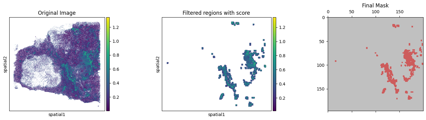
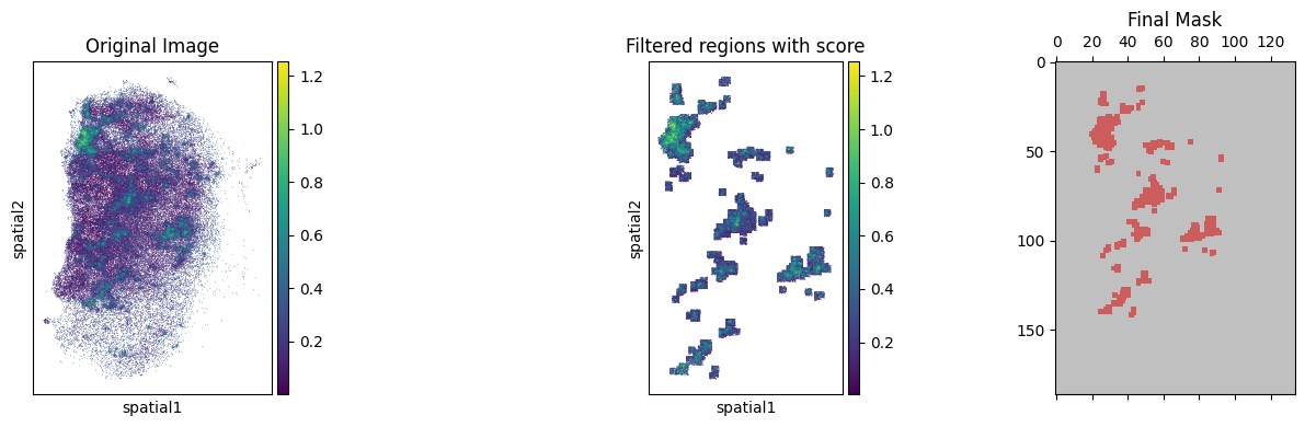
Step2-1: Batch processing samples

Using KDE algorithm to select the smoothed region with high B-cell score

adata = BAITS.st.tl.batch_process( 
    
    adata=adata, sample_name=sample_name, score_name=score_name,   
    processing_func = BAITS.st.tl.kde_filter, 
    verbose=True,
    func_kwargs={ 'score_name':score_name, 'high_binSize': 100, 'default_thread_num': 36, 'clean_mask_size': (3,3)}
)

🔬 Start process sample:	P1121_LM
🔎 Step 1 - Process data:		0.79 s
📊 Spatial cell number to evaluate:		39400
🏋️ Step 2 - KDE scoring:		335.07 s
📊 Using 90 th percentile threshold:		0.000
🔬 Step 3 - Obtain correct coords:		0.27 s
🎨 Plot results
✅ Sample: P1121_LM done!



🔬 Start process sample:	P0516_LM
🔎 Step 1 - Process data:		0.09 s
📊 Spatial cell number to evaluate:		25058
🏋️ Step 2 - KDE scoring:		67.96 s
📊 Using 90 th percentile threshold:		0.000
🔬 Step 3 - Obtain correct coords:		0.10 s
🎨 Plot results
✅ Sample: P0516_LM done!

adata

AnnData object with n_obs × n_vars = 968003 × 25091
    obs: 'n_genes_by_counts', 'total_counts', 'pct_counts_mt', 'celltype', 'sample', 'Bcell_enrichment', 'filtered_coords'
    obsm: 'spatial'

Using DBscan algorithm to cluster sinle BLA region

adata = BAITS.st.tl.batch_process( 
    
    adata=adata, sample_name=sample_name, score_name=score_name,   
    processing_func=BAITS.st.tl.dbscan_cluster, 
    verbose=True,
    func_kwargs={ 'eps': 100, 'min_samples': 50 } 
)

🔬 Start process sample:	P1121_LM
✅ Sample: P1121_LM done!



🔬 Start process sample:	P0516_LM
✅ Sample: P0516_LM done!

Step2-2: Processing samples one by one (Optional)

To enable sample-specific fine-tuning, users can perform BAITS analysis on individual samples.

The analytical procedure is identical to the batch process described in Step 2-1; users may select their preferred configuration method.

# By using function **BAITS.st.tl.kde_filter**, we could filter cells with low B-cell-score

filtered_adata = []

for sample in ['P0516_LM']:
    print('Sample:\t', sample)
    tmp_ad = adata[adata.obs[sample_name]==sample].copy()
    tmp_res = BAITS.st.tl.kde_filter(tmp_ad, score_name=score_name, plot=True, threshold_method='percentile', custom_threshold=90) 
    
    filtered_adata.append(tmp_res)

Sample:	 P0516_LM
🔎 Step 1 - Process data:		0.09 s
📊 Spatial cell number to evaluate:		25058
🏋️ Step 2 - KDE scoring:		66.45 s
📊 Using 90 th percentile threshold:		0.000
🔬 Step 3 - Obtain correct coords:		0.17 s
🎨 Plot results

adata = ad.concat(filtered_adata)
adata

AnnData object with n_obs × n_vars = 347386 × 25091
    obs: 'n_genes_by_counts', 'total_counts', 'pct_counts_mt', 'celltype', 'sample', 'Bcell_enrichment', 'filtered_coords', 'BLA_id'
    obsm: 'spatial'

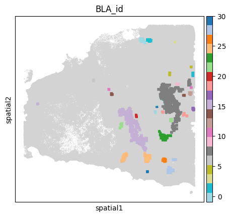
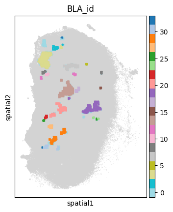
# **st.tl.dbscan_filter** employs the DBSCAN algorithm to identify spatially contiguous cellular domains into BLA.

res_adata = []

for sample in ['P0516_LM']:
    print('Sample:\t', sample)
    sample_ad = adata[adata.obs[sample_name]==sample].copy()
    
    # select region with high B cell score
    tmp_ad = sample_ad[sample_ad.obs['filtered_coords']].copy()
    tmp_res = BAITS.st.tl.dbscan_cluster(tmp_ad)
    
    sample_ad.obs['BLA_id'] = np.nan
    sample_ad.obs.loc[tmp_res.obs.index, 'BLA_id'] = tmp_res.obs['BLA_id']

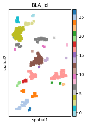
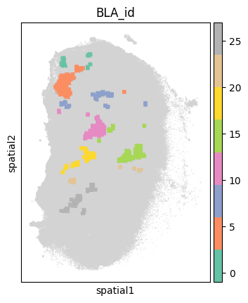
    sc.pl.spatial(sample_ad, color='BLA_id', spot_size=50, cmap='Set2',
                      legend_fontsize='medium', legend_fontweight='normal',  title='BLA_id', legend_loc='on data')
    
    res_adata.append(sample_ad)

Sample:	 P0516_LM