BAITS.SR module

import os

import numpy as np
import pandas as pd
import matplotlib.pyplot as plt
import seaborn as sns
from scipy.stats import pearsonr
import matplotlib.pyplot as plt
import matplotlib.image as mpimg

import BAITS

Import files

Users could read the example data from the github, also could access the data through the link

bcr_loc_df = pd.read_csv('./data/bcr_rep_loc_sampled.tsv', sep='\t',index_col=0)

bcr_loc_df.head()

	sample	bcUmi	clone	aaClone	Vgene	Jgene	Cgene	X	Y	spatial_cluster	tissue_region	InAggOrNot	Bcell_aggregate_label	BaggArea	celltype
0	P0516-LM	E14D5FEFEBE3D5C47	TGTCAACAGAGTCACAGTATACCTACTTTT_CQQSHSIPTF_IGKV...	CQQSHSIPTF_IGKV1-39_IGKJ2_IGK	IGKV1-39	IGKJ2	IGK	11873	3350	C4: TLS-like	Peri-tumor	InAgg	P0516_LM-12	1789700.0	B
1	P0516-LM	8E153B79054792CA2	TGTCAACAATATAGCACTGTCCCCCTCACTTTC_CQQYSTVPLTF_...	CQQYSTVPLTF_IGKV1-27_IGKJ4_IGK	IGKV1-27	IGKJ4	IGK	7616	5287	C4: TLS-like	Adjacent-tissue	InAgg	P0516_LM-12	1789700.0	B
2	P0516-LM	CF7AAA1CE45FCED95	TGTCAGCAATATTATGGTCTTCCATTCAGTTTG_CQQYYGLPFSL_...	CQQYYGLPFSL_IGKV4-1_IGKJ3_IGK	IGKV4-1	IGKJ3	IGK	4077	2350	C3: Plasma enriched	Adjacent-tissue	InAgg	P0516_LM-0	1098000.0	Plasma
3	P0516-LM	67DE18BD6C145817C	TGTCAGCAGTTTCACAACTGGCCCTACACATTT_CQQFHNWPYTF_...	CQQFHNWPYTF_IGKV3-15_IGKJ2_IGK	IGKV3-15	IGKJ2	IGK	7390	5312	C2: Macrophages enriched	Adjacent-tissue	InAgg	P0516_LM-12	1789700.0	Hepatocytes
4	P0516-LM	353E0FEC9BEE66A22	TGTCAACAGTCCGCAAGTATTCCGTGGACGTTC_CQQSASIPWTF_...	CQQSASIPWTF_IGKV4-1_IGKJ1_IGK	IGKV4-1	IGKJ1	IGK	4380	2441	C3: Plasma enriched	Adjacent-tissue	InAgg	P0516_LM-0	1098000.0	B

Define parameters

sample_col = 'sample'
Umi_col = 'bcUmi'
clone_col = 'clone'
cdr3nt_col = 'cdr3nt'

Vgene_col = 'Vgene'
Jgene_col = 'Jgene'
Cgene_col = 'Cgene'

loc_x_col = 'X'
loc_y_col='Y'

Quality Control

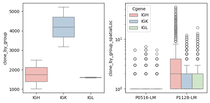
Compute the clone number and UMIs of spatial location (at the bin1 level)

bcr_loc_df = BAITS.VDJ.tl.calculate_qc_clones( bcr_loc_df, sample_col, Cgene_col, clone_col, loc_x_col=loc_x_col, loc_y_col=loc_y_col, plot=True ) 

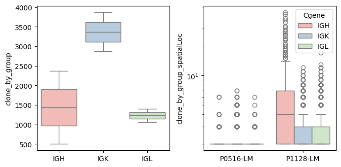
bcr_loc_df = BAITS.VDJ.tl.filter_clones_spatial(bcr_loc_df, 'clone_by_group_spatialLoc', min_clone_spatial=1)
bcr_loc_df = BAITS.VDJ.tl.calculate_qc_clones( bcr_loc_df, sample_col, Cgene_col, clone_col, plot=True ) 

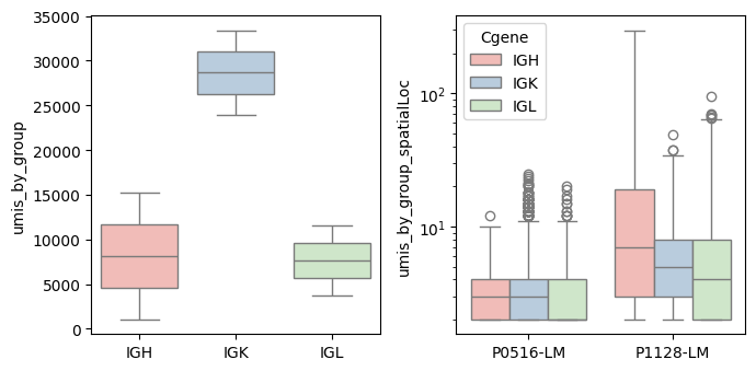
bcr_loc_df = BAITS.VDJ.tl.calculate_qc_umis( bcr_loc_df, sample_col, Cgene_col, clone_col, plot=False ) 

bcr_loc_df = BAITS.VDJ.tl.filter_umi_spatial(bcr_loc_df, 'umis_by_group_spatialLoc', min_umi_spatial=1)
bcr_loc_df = BAITS.VDJ.tl.calculate_qc_umis( bcr_loc_df, sample_col, Cgene_col, clone_col, plot=True ) 

Spatial repertoire feature

For user-defined spatial regions of interest, such as B cell aggregates (BLAs) and other specialized spatial niches, this module calculates the full suite of BCR repertoire features introduced in the BAITS-IR module.

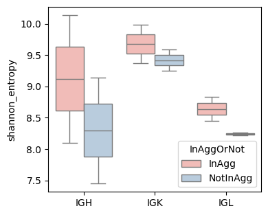
shannon_entropy (based on spatial location

groups = [sample_col, Cgene_col, 'InAggOrNot']
shannon_entropy_df = BAITS.VDJ.tl.compute_grouped_index(bcr_loc_df, sample_col, Cgene_col, clone_col, groups, loc_x_col=loc_x_col, loc_y_col=loc_y_col, index='shannon_entropy')

fig, ax = plt.subplots(1,1,figsize=(4, 3.5))
BAITS.VDJ.pl._boxplot(shannon_entropy_df, 'Cgene', 'shannon_entropy', groupby='InAggOrNot', palette='Pastel1', xlabel=None, ylabel='shannon_entropy', log=False, ax=ax )
plt.show()

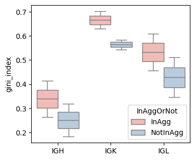
gini_index (based on spatial location

groups = [sample_col, Cgene_col, 'InAggOrNot']
gini_index_df = BAITS.VDJ.tl.compute_grouped_index(bcr_loc_df, sample_col, Cgene_col, clone_col, groups, loc_x_col=loc_x_col, loc_y_col=loc_y_col, index='gini_index')

fig, ax = plt.subplots(1,1,figsize=(4, 3.5))
BAITS.VDJ.pl._boxplot(gini_index_df, 'Cgene', 'gini_index', groupby='InAggOrNot', palette='Pastel1', xlabel=None, ylabel='gini_index', log=False, ax=ax )
plt.show()

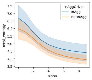
renyi_entropy (based on spatoal location

groups = [sample_col, Cgene_col, 'InAggOrNot']
renyi_entropy_df =  BAITS.VDJ.tl.compute_grouped_index(bcr_loc_df, sample_col, Cgene_col, clone_col, groups, loc_x_col=loc_x_col, loc_y_col=loc_y_col, index='renyi_entropy')

fig, ax = plt.subplots(1,1,figsize=(4, 3.5))
sns.lineplot(data=renyi_entropy_df[renyi_entropy_df[Cgene_col]=='IGH'], x="alpha", y="renyi_entropy", hue='InAggOrNot', ax=ax )
plt.show()

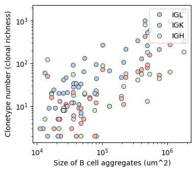
Corrlation between computed_index and the area of the B_aggregates

agg_clone_df = BAITS.VDJ.tl.calculate_qc_clones( bcr_loc_df, 'Bcell_aggregate_label', Cgene_col, clone_col, plot=False ) 

plot_df = agg_clone_df[['sample', 'Cgene', 'BaggArea','clone_by_group']].drop_duplicates().dropna() 

fig, ax = plt.subplots(1,1,figsize=(4, 3.5))
BAITS.VDJ.pl._scatter_plot(plot_df, 'BaggArea', 'clone_by_group', groupby='Cgene', palette='Pastel1', x_log=True, y_log=True, 
             xlabel='Size of B cell aggregates (um^2)', ylabel='Clonetype number (clonal richness)', ax=ax )
plt.show()

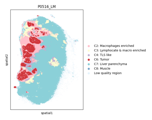
Clonal migration

In the tutorial “st_spatial_cluster”, we define the niches within a region through spatial clustering, as illustrated below:

img = mpimg.imread('/home/zhaoyp/1.CRLM_XCR/BAITS/docs/data/P0516_LM_spatialCluster_umap.png')   
plt.imshow(img)
plt.axis('off')   
plt.show()

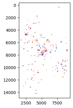
By the way, we also could visualize the spatial distribution of VDJ sequences, as illustrated below:

BAITS.VDJ.pl._plot_xcr( bcr_loc_df[(bcr_loc_df[sample_col]=='P0516-LM') & (bcr_loc_df[Cgene_col]=='IGH')], clone_col,loc_x_col, loc_y_col ) 

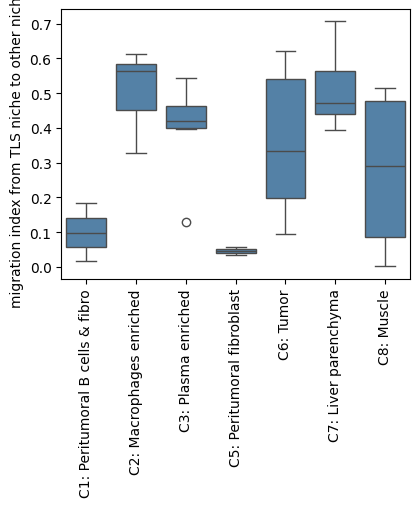
Based on spatial niches and VDJ distribution, we could use spatial migration index to quantify the BCR ‘migration’ patten.

migr_df = BAITS.VDJ.tl.compute_migraIdx(bcr_loc_df, sample_col='sample', clone_col='clone', chain_col='Cgene', cluster_col='spatial_cluster', x_col='X', y_col='Y')

The clonal migration index from the TLS region to other niches is visualized here.

tls_to_otherNiche = migr_df[migr_df['cluster_source']=='C4: TLS-like'].sort_values('cluster_target').copy()

plt.subplots(1, 1, figsize=(4.5, 3.5))
sns.boxplot(data=tls_to_otherNiche, x='cluster_target', y='BCR_cross',color='steelblue')
plt.xticks(rotation=90)
plt.ylabel('migration index from TLS niche to other niches') 
plt.xlabel('')
plt.show()

Clonal niche analysis

To investigate the spatial niche surrounding the specific clone, we filtered the most expanded clones.

bcr_loc_df[['sample','aaClone']].value_counts().head(2)

sample    aaClone                          
P0516-LM  CQQYHDLPITF_IGKV1-33_IGKJ5_IGK       2132
          CQQSYRTPRLLFTF_IGKV1-39_IGKJ3_IGK    1471
dtype: int64

Here, we investigate the spatial niche surrounding the most expanded clone, ‘CQQYHDLPITF_IGKV1-33_IGKJ5_IGK’, in sample ‘P0516-LM’.

data_out, niche_prop, niche_count = BAITS.VDJ.tl.calculate_clone_niche(
    bcr_loc_df,
    sample="P0516-LM",
    target_clone="CQQYHDLPITF_IGKV1-33_IGKJ5_IGK",
    radius=50, # um
    scale=2    # In Stereo-seq, the length of each spot is 0.5 um
)

import matplotlib.pyplot as plt
import seaborn as sns

fig, ax = plt.subplots(1, 1, figsize=(4.5, 3.5))

sns.barplot(x=niche_prop.index, y=niche_prop.values, color='steelblue', ax=ax)

ax.set_ylabel('Surrounding cell type proportion')
ax.set_xlabel('')
plt.xticks(rotation=90)

for i, v in enumerate(niche_prop.values):
    ax.text( i, v + 0.005, f"{v:.2f}", ha='center',va='bottom',fontsize=9)

plt.tight_layout()
plt.show()

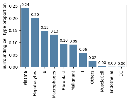
Here, we observe that the most abundant cell type surrounding the clone ‘CQQYHDLPITF_IGKV1-33_IGKJ5_IGK’ in sample ‘P0516-LM’ is ‘plasma’, followed by ‘hepatocytes’.